Chapter 7 Neural Network
By Eliana Perea Barreto
7.1 Overview
Neural networks are computational models inspired by the workings of the human brain. The base-units of these networks are neurons, which are essentially units of value that exist within a system of layers. In each layer, the neurons are properly activated and managed to determine the strength and direction of the signals transmitted between them. The process of activating neurons to achieve coherent outputs is governed by weights and biases, which control the flow and transformation of input data through the network.
7.2 Algorithmic Framework
The neural network consists of neurons, weights, biases, and layers. These elements collectively form its architecture. The quantity of these components depend on the model’s complexity and desired precision, ranging from simple (a few layers and neurons) to highly intricate structures (thousands of neurons and numerous layers). In this specific case, a simple neural network is employed to predict flights arrival delay (arr_delay) based on carrier names (carrier). At the core of the model, there are 4 layers: the input layer (x) with 16 neurons (one for each carrier), 2 hidden layers (z_1, z_2) with 3 and 2 neurons respectively, and the output layer (y) with one neuron.
Layers
# Initialize layers
input_size <- 16
hidden_size1 <- 3
hidden_size2 <- 2
output_size <- 1
As carrier names are categorical variables, they must be encoded into numeric format. For that, one-hot encoding is implemented to convert the categorical carrier feature into multiple binary features. The goal is to prevent the model from assuming any ordinal relationship between the categories. Each row will have a 1 in the column corresponding to its carrier and 0 in the others.
One-Hot Encode
Information is transmitted in this model through the activation of the neurons in each layer. Now, imagine activating all neurons simultaneously would result in a chaotic mix of unrelated information. To address this, “weights”; values tare set randomly at the beginning of the process but are adjusted over time to minimize prediction errors. As Neural networks operate through matrix operations, 3 weight matrices are generated to contain the weighted values of each layer.
Weights
# Initialize weights
W1 <- matrix(rnorm(input_size * hidden_size1), nrow=input_size, ncol=hidden_size1)
W2 <- matrix(rnorm(hidden_size1 * hidden_size2), nrow=hidden_size1, ncol=hidden_size2)
W3 <- matrix(rnorm(hidden_size2 * output_size), nrow=hidden_size2, ncol=output_size)
As the information flows between the network’s layers through the activation of neurons with weights, the biases (b) supports each layer by accounting for any inherent offsets in the data, allowing the model to better fit the training examples.
Bias
# Initialize biases
b1 <- matrix(rnorm(hidden_size1), nrow=1, ncol=hidden_size1)
b2 <- matrix(rnorm(hidden_size2), nrow=1, ncol=hidden_size2)
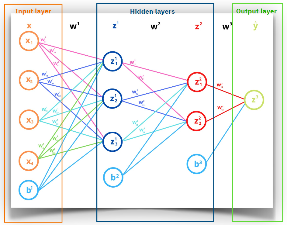
b3 <- matrix(rnorm(output_size), nrow=1, ncol=output_size)Below is a visual representation of the architecture of this neural network. For simplicity, the input layer is depicted with only 4 neurons. However, it is important to note that this model actually starts with 16 neurons in the input layer:
7.3 Training & Predicting Process
Normally in a training/testing predicting process the the data is split in 2 sets. 80% of the data is allocated for model fitting while the remaining 20% is reserved for the evaluation the model’s predictive accuracy.
# Split the data (80% training, 20% testing)
indices <- sample(1:nrow(datat), 0.8 * nrow(data))
train_data <- data_flight[indices, ]
test_data <- data_flight[-indices, ]
7.3.1 Feed-forward Algorithm
Referring back to the visual representation of the model’s structure from the previous chapter, it’s possible conceptualize the mathematical formula for the first hidden layer (\(Z^{1}\)) as a linear combination of neurons in the input layer (\(X\)) the weights’ matrix (\(W^{1}\)) plus the bias \(b^{1}\):
\[ Z^{1} = X \cdot W^{1} + b^{1} \]
This formula is at the core of the forward pass where transmitted inputs through the network’s layer result in a predicted output. As the process moves forwards, the components of that formula are replaced by values corresponding to each layer. Additionally, the output of each layer must be normalized before it is transmitted to the next layer, in order to produce a cohesive result and also to facilitate the network’s ability to generalize. This normalization process is carried out by an activation function such Sigmoid or ReLU. In this specific case, Sigmoid squishification is implemented to take the weighted sum of the neurons and squish it into a range between 0 and 1. Basically, in this logistic function negative inputs end up close to zero, positive inputs get closed to one.\[ \sigma(x) = \frac{1}{1 + e^{-x}} \]
When \(x\) is a large negative number, \(e^{-x}\) becomes very large. Example, \(x = -10, e^{-(-10)} = e^{10}\). Then, this value will do the fraction \(\frac{1}{1+e^{10}}\) very small, approaching zero.
With all components defined, the forward pass can be initiated. Additionally, a Cost function is set to measure the network’s performance. This Cost function (also called Loss function) quantifies the error between the predicted output (\(\hat{y}\)) and the actual output (\(y\)). In this exercise, the Cost function is the Mean Squared Error (MSE).
\[ L(\hat{y}, y) = (\hat{y} - y)^2 \]
# Feed-forward
input <- train_data[, -ncol(train_data)]
Z1_train <- as.matrix(input) %*% W1 + matrix(b1, nrow=nrow(train_data), ncol=ncol(b1))
A1_train <- sigmoid(Z1_train)
Z2_train <- A1_train %*% W2 + matrix(b2, nrow = nrow(A1_train), ncol = ncol(b2))
A2_train <- sigmoid(Z2_train)

# No activation function for the last layer as this is a regression problem
Z3_train <- A2_train %*% W3 + matrix(b3, nrow = nrow(A2_train), ncol = ncol(b3))
predicted_output_train <- Z3_train

# Calculate mean squared error for training data
cost_train <- mean((predicted_output_train - train_data$arr_delay)^2)
## Cost previous to iterations: 1973.661
## AVG Cost per sample: 0.5068467The high total cost indicates that the predictions are far from the actual values, which is expected since the model hasn’t undergone any training iterations yet. The learning abilities of Neural Networks highly rely in an iterative process to adjust the weights. To enhance the model’s performance, we need to define the number of training cycles, or epochs. Here, we set the number of epochs to 10, but this can be adjusted based on the model’s prediction accuracy.
epochs <- 10Additionally all the operations presented till now constitute only one section of the learning process. The cost is high because the model hasn’t received any clues to establish the correct direction to minimize the Cost, which is the ultimate goal of this process. To achieve it, the gradient of the cost function must be calculated.
7.3.2 Backpropagation
Self-training in machine learning refers to a model’s ability to iteratively analyze input data and learn to improve performance. In Backpropagation, the process is carried out backward, transmitting the error between predicted and actual outputs to previous layers. This adjusts weights and biases, minimizing the cost function.
Minimization occurs when the model identifies the direction to reduce the cost, guided by the gradient of the cost function. If the slope is positive, moving in the negative gradient direction decreases the cost, and viceversa if the slope is negative.
Mathematically, partial derivatives determine the gradient. The partial derivative of the cost function with respect to weights is denoted as \(\frac{\partial Cost}{ \partial W^{(L)}}\). The weights are related to the values of a previous layer’s weighted input \(Z^{(L)}\)and its activation function \(a^{(L)}\)
The derivative of \(Z^{(L)}\) with respect to \(W^{(L)}\) is \(\frac{\partial Z^{(L)}}{\partial W^{(L)}} = a^{(L-1)}\)
The derivative of the activation function \(a^{(L)}\) with respect to \(Z^{(L)}\) is \(\frac{\partial a^{(L)}}{\partial Z^{(L)}} = \sigma'(Z^{(L)})\)
The derivative of the cost with respect to the activation \(a^{(L)}\) is \(\frac{\partial Cost}{\partial a^{(L)}} = 2 (a^{(L)} - y)\).
Therefore, the formula for Backpropagation can be defined as follows:
\[ \frac{\partial Cost}{\partial W^{(L)}} = \frac{\partial Z^{(L)}}{\partial W^{(L)}} \cdot \frac{\partial a^{(L)}}{\partial Z^{(L)}} \cdot \frac{\partial Cost }{\partial a^{(L)}} \]
Before initiating the code for Backpropagation, the derivative of the sigmoid function is defined:
Sigmoid Derivative
dZ3_train <- 2 * (predicted_output_train - train_data$arr_delay)
dW3 <- t(A2_train) %*% dZ3_train # First multiplication
dA2_train <- dZ3_train %*% t(W3) # First error propagation

dZ2_train <- dA2_train * sigmoid_derivative(Z2_train)
dW2 <- t(A1_train) %*% dZ2_train # Second multiplication
dA1_train <- dZ2_train %*% t(W2) # Second error propagation

dZ1_train <- dA1_train * sigmoid_derivative(Z1_train)
dW1 <- t(input) %*% dZ1_train # Third multiplication
The process is concluded with the update of the weights which, in gradient descent, is given by the formula:
\[W^{(L)} \leftarrow W^{(L)} - \eta \frac{\partial Cost}{\partial W^{(L)}}\]
where \(\eta\) is the learning ratio, set to 0.01 in this specific case. The learning rate controls the size of the adjustments made to the model’s weights during training. A learning rate of 0.01 indicates that the weights are updated in small increments, which helps in gradually minimizing the error without overshooting the optimal values.
learning_rate = 0.01 Update
With that, the explanation of the neural network training process is concluded. The remaining task is to iterate over this process repeatedly to refine the model’s performance. In our case, the model will undergo 10 iterations, as the number of epochs was initially set to that value. To view the implementation of the full code with these iterations, click on Code Preview.
Code Preview
# Training loop function with adjusted learning rate
train_model <- function(train_data, W1, W2, W3, b1, b2, b3, epochs, learning_rate) {
for (epoch in 1:epochs) {
input <- train_data[, -ncol(train_data)]
Z1_train <- as.matrix(input) %*% W1 + matrix(b1, nrow=nrow(train_data), ncol=ncol(b1))
A1_train <- sigmoid(Z1_train)
Z2_train <- A1_train %*% W2 + matrix(b2, nrow = nrow(A1_train), ncol = ncol(b2))
A2_train <- sigmoid(Z2_train)
Z3_train <- A2_train %*% W3 + matrix(b3, nrow = nrow(A2_train), ncol = ncol(b3))
predicted_output_train <- Z3_train
# Calculate mean squared error for training data
loss_train <- mean((predicted_output_train - train_data$arr_delay)^2)
dZ3_train <- 2 * (predicted_output_train - train_data$arr_delay)
dW3 <- t(A2_train) %*% dZ3_train # First multiplication
dA2_train <- dZ3_train %*% t(W3) # First error propagation
dZ2_train <- dA2_train * sigmoid_derivative(Z2_train)
dW2 <- t(A1_train) %*% dZ2_train # Second multiplication
dA1_train <- dZ2_train %*% t(W2) # Second error propagation
dZ1_train <- dA1_train * sigmoid_derivative(Z1_train)
dW1 <- t(input) %*% dZ1_train # Third multiplication
# Bias
db3 <- colSums(dZ3_train)
db2 <- colSums(dZ2_train)
db1 <- colSums(dZ1_train)
# Gradient Clipping. to prevent gradient becoming to large
clip_value <- 5000
dW3 <- pmax(pmin(dW3, clip_value), -clip_value)
dW2 <- pmax(pmin(dW2, clip_value), -clip_value)
dW1 <- pmax(pmin(dW1, clip_value), -clip_value)
db3 <- pmax(pmin(db3, clip_value), -clip_value)
db2 <- pmax(pmin(db2, clip_value), -clip_value)
db1 <- pmax(pmin(db1, clip_value), -clip_value)
# Update of weights and bias
W3 <- W3 - learning_rate * dW3
b3 <- b3 - learning_rate * db3
W2 <- W2 - learning_rate * dW2
b2 <- b2 - learning_rate * db2
W1 <- W1 - learning_rate * dW1
b1 <- b1 - learning_rate * db1
# Print loss for monitoring
cat("Epoch:", epoch, " - Loss (Training):", loss_train, "\n")
}
list(W1 = W1, W2 = W2, W3 = W3, b1 = b1, b2 = b2, b3 = b3)
}
# Call the train_model function with the adjusted learning rate
updated_parameters <- train_model(train_data,
W1, W2, W3,
b1, b2, b3,
epochs,
learning_rate)## Epoch: 1 - Loss (Training): 2002.533
## Epoch: 2 - Loss (Training): 1939.68
## Epoch: 3 - Loss (Training): 1837.457
## Epoch: 4 - Loss (Training): 1739.89
## Epoch: 5 - Loss (Training): 1678.186
## Epoch: 6 - Loss (Training): 1873.737
## Epoch: 7 - Loss (Training): 2213.296
## Epoch: 8 - Loss (Training): 1621.107
## Epoch: 9 - Loss (Training): 1581.032
## Epoch: 10 - Loss (Training): 1541.294
## Epoch: 11 - Loss (Training): 1501.356
## Epoch: 12 - Loss (Training): 1462.962
## Epoch: 13 - Loss (Training): 1600.802
## Epoch: 14 - Loss (Training): 1394.36
## Epoch: 15 - Loss (Training): 1790.194
## Epoch: 16 - Loss (Training): 1392.42
## Epoch: 17 - Loss (Training): 1728.941
## Epoch: 18 - Loss (Training): 1301.008
## Epoch: 19 - Loss (Training): 1695.775
## Epoch: 20 - Loss (Training): 1253.605
## Epoch: 21 - Loss (Training): 1659.647
## Epoch: 22 - Loss (Training): 1221.139
## Epoch: 23 - Loss (Training): 1631.177
## Epoch: 24 - Loss (Training): 1163.037
## Epoch: 25 - Loss (Training): 1654.488
## Epoch: 26 - Loss (Training): 1135.523
## Epoch: 27 - Loss (Training): 1635.576
## Epoch: 28 - Loss (Training): 1110.887
## Epoch: 29 - Loss (Training): 1618.336
## Epoch: 30 - Loss (Training): 1092.078
## Epoch: 31 - Loss (Training): 1527.634
## Epoch: 32 - Loss (Training): 1089.671
## Epoch: 33 - Loss (Training): 1504.699
## Epoch: 34 - Loss (Training): 1073.576
## Epoch: 35 - Loss (Training): 1483.005
## Epoch: 36 - Loss (Training): 1058.288
## Epoch: 37 - Loss (Training): 1467.154
## Epoch: 38 - Loss (Training): 1049.159
## Epoch: 39 - Loss (Training): 1451.484
## Epoch: 40 - Loss (Training): 1038.714
## Epoch: 41 - Loss (Training): 1439.32
## Epoch: 42 - Loss (Training): 1040.032
## Epoch: 43 - Loss (Training): 1428.715
## Epoch: 44 - Loss (Training): 1037.947
## Epoch: 45 - Loss (Training): 1416.46
## Epoch: 46 - Loss (Training): 1028.57
## Epoch: 47 - Loss (Training): 2336.064
## Epoch: 48 - Loss (Training): 1097.746
## Epoch: 49 - Loss (Training): 1085.115
## Epoch: 50 - Loss (Training): 988.8929
## Epoch: 51 - Loss (Training): 1034.588
## Epoch: 52 - Loss (Training): 1088.998
## Epoch: 53 - Loss (Training): 1024.318
## Epoch: 54 - Loss (Training): 987.7465
## Epoch: 55 - Loss (Training): 986.9891
## Epoch: 56 - Loss (Training): 1103.72
## Epoch: 57 - Loss (Training): 976.7364
## Epoch: 58 - Loss (Training): 1098.627
## Epoch: 59 - Loss (Training): 969.0878
## Epoch: 60 - Loss (Training): 1097.695
## Epoch: 61 - Loss (Training): 960.647
## Epoch: 62 - Loss (Training): 1099.25
## Epoch: 63 - Loss (Training): 952.2167
## Epoch: 64 - Loss (Training): 1102.652
## Epoch: 65 - Loss (Training): 945.6094
## Epoch: 66 - Loss (Training): 1006.211
## Epoch: 67 - Loss (Training): 939.0979
## Epoch: 68 - Loss (Training): 1110.306
## Epoch: 69 - Loss (Training): 932.8845
## Epoch: 70 - Loss (Training): 1113.977
## Epoch: 71 - Loss (Training): 929.0473
## Epoch: 72 - Loss (Training): 1013.099
## Epoch: 73 - Loss (Training): 914.9852
## Epoch: 74 - Loss (Training): 1047.083
## Epoch: 75 - Loss (Training): 914.3144
## Epoch: 76 - Loss (Training): 1037.97
## Epoch: 77 - Loss (Training): 914.2082
## Epoch: 78 - Loss (Training): 1155.68
## Epoch: 79 - Loss (Training): 912.1165
## Epoch: 80 - Loss (Training): 1031.937
## Epoch: 81 - Loss (Training): 910.0517
## Epoch: 82 - Loss (Training): 1028.026
## Epoch: 83 - Loss (Training): 909.1717
## Epoch: 84 - Loss (Training): 1018.629
## Epoch: 85 - Loss (Training): 908.0742
## Epoch: 86 - Loss (Training): 1014.12
## Epoch: 87 - Loss (Training): 905.119
## Epoch: 88 - Loss (Training): 1011.756
## Epoch: 89 - Loss (Training): 905.4758
## Epoch: 90 - Loss (Training): 1008.495
## Epoch: 91 - Loss (Training): 904.4414
## Epoch: 92 - Loss (Training): 1001.232
## Epoch: 93 - Loss (Training): 927.811
## Epoch: 94 - Loss (Training): 999.2898
## Epoch: 95 - Loss (Training): 904.6963
## Epoch: 96 - Loss (Training): 995.6421
## Epoch: 97 - Loss (Training): 925.984
## Epoch: 98 - Loss (Training): 994.6018
## Epoch: 99 - Loss (Training): 897.3991
Initially, with 10 epochs and a learning rate of 0.01, the training process showed signs of divergence.This means that the loss was increasing exponentially instead of decreasing, which is the opposite of what should ideally happen. To address this issue, the learning rate was adjusted to 0.0002 to ensure more gradual updates to the model weights. Additionally, the weight matrices were normalized with a mean of 0 and a standard deviation of 0.01. The number of epochs was extended to 99 and gradient clipping was set to prevent the gradients from getting too large. Here are some observations based on the provided results:
Convergence: The loss was decreasing rapidly after the clip value was set to 5000. The last achieve value is around 897.3. This indicates that the model has converged. Further training epochs might be needed to significant improvements in the loss.
Stability: Generally the loss has a tendency to decrease, however there are intermittent value fluctuations.
Learning Rate: The chosen learning rate of 0.0002 seems to be appropriate for the training process, allowing the model to make consistent progress in reducing the loss over the epochs.
Effectiveness: The final loss achieved after 99 epochs, indicating that the model has learned from the data effectively.
A Feed-forward architecture is created to assess the model’s predictive abilities with the testing data.
Predict model
predict_model <- function(test_data, W1, W2, W3, b1, b2, b3) {
  input <- test_data[, -ncol(test_data)]
  Z1_test <- as.matrix(input) %*% W1 + matrix(b1, nrow=nrow(test_data), ncol=ncol(b1))
  A1_test <- sigmoid(Z1_test)
  Z2_test <- A1_test %*% W2 + matrix(b2, nrow=nrow(A1_test), ncol=ncol(b2))
  A2_test <- sigmoid(Z2_test)
  Z3_test <- A2_test %*% W3 + matrix(b3, nrow=nrow(A2_test), ncol=ncol(b3))
  predicted_output_test <- Z3_test
  return(predicted_output_test)
}
The model exhibits promise in capturing the variance within the data, as indicated by the substantial decrease in loss during both training and testing phases. This implies that the model has the capacity to learn from the provided data and make predictions effectively. The rapid decline in loss throughout the established epochs suggests that further iterations could enhance the model’s capabilities, indicating room for improvement with additional training epochs.
Moreover, fluctuations observed in loss during both training and testing phases suggest potential instability or heightened sensitivity, likely stemming from the relatively small dataset size. With fewer data points, the model may be more vulnerable to noise or outliers, increasing the risk of overfitting. I tried to address this issue by normalizing the training and testing data, however the fluctuations persisted. This highlights the need for further exploration and refinement of the model architecture. Additional regularization techniques might be considered, such as fine-tuning hyperparameters or employing methods like Lasso regression to effectively mitigate the issue of fluctuation and improve the model’s performance.
7.4 Strengths & Limitations
7.4.1 Strengths
Neural networks can model complex, non-linear relationships in data, capturing patterns that simpler models might miss. They also benefit from parallel processing capabilities which makes them efficient for large-scale data processing. Despite their complexity, neural networks can provide insights into the relationships between input features and target variables, aiding in the interpretation of learned patterns and relationships. When trained properly, they generalize well to new, unseen data, offering robust and reliable predictions.Additionally, neural networks are suitable for a wide range of applications, allowing them to tackle diverse problem domains.
Lastly, they have a flexible architecture that allows for experimentation with different configurations, including the number of layers, neurons and activation functions. This flexibility enables the tailoring of models to specific tasks and data characteristics. Moreover, neural networks can automatically learn features from raw data, reducing the need for manual feature engineering.
7.4.2 Limitations
Despite their strengths, neural networks have several limitations that can hinder their performance and applicability. One major limitation is their requirement for large datasets. Neural networks need vast amounts of labeled data to train effectively, which can be a significant barrier in domains where data is scarce. Additionally, they are computationally intensive, requiring powerful GPUs and large memory for training, which can be a constraint in some environments.
The complexity and interpretability of neural networks are also significant challenges. As model architectures become more complex, they often turn into “black boxes,” making it difficult to understand how decisions are made. This decreased interpretability can be problematic in applications where understanding the decision-making process is crucial. Furthermore, neural networks are vulnerable to small perturbations to input data which can lead to significant errors in predictions.