Chapter 2 Simple Linear Model
By Sheptim Veseli
2.1 Introduction
This analysis investigates the impact of airline carriers on flight arrival delays using the nycflights13 dataset. The dataset contains flight details for all aircraft departing from New York City airports throughout 2013. The objective is to explore the predictive potential of a simple linear regression model, where the arrival delay (arr_delay) is the dependent variable and the carrier (airline name) is the primary independent variable.
2.2 Data Preparation
The original dataset comprises 336,776 entries across 19 variables. To meet the project’s criteria of working with a dataset within a range of 10^3 to 10^5 rows, a random sample of 5000 entries was selected. Additionally, rows with missing values in key variables (dep_time, arr_time, arr_delay, tailnum, air_time) were removed, resulting in a cleaned dataset of 2052 rows.
Code Preview
# Set random seed to ensure reproducibility
set.seed(123)

# Randomly select 5000 row indices and use them to subset original data
selected_indices <- sample(1:nrow(flights), 5000, replace = FALSE)
flights_subset <- flights[selected_indices, ]

# Remove rows with missing values in key variables
flights_subset <- flights_subset[complete.cases(flights_subset$dep_time, flights_subset$arr_time, flights_subset$arr_delay, flights_subset$tailnum, flights_subset$air_time), ]

# Remove negative values from arrival delay time (arr_delay)
flights_subset <- flights_subset[flights_subset$arr_delay >= 0, ]

# Apply logarithmic transformation to arrival delay time (arr_delay)
flights_subset$log_arr_delay <- log(flights_subset$arr_delay + 1)
2.3 Descriptive Statistics
Descriptive statistics provide a summary of the data’s main characteristics, offering insight into the central tendency, dispersion, and distribution of the dataset. For this analysis, we focus on two key aspects: arrival delays and the distribution of flights among different carriers.
2.3.1 Arrival Delay Statistics
The arrival delay data reveals insightful characteristics of flight punctuality.
##    Min. 1st Qu.  Median    Mean 3rd Qu.    Max.
##    0.00    7.00   19.00   37.06   46.00  681.00
The minimum recorded delay is 0 minutes, indicating that some flights arrived precisely on schedule or even earlier. The first quartile (25th percentile) value is 7 minutes, suggesting that 25% of the flights experienced delays of 7 minutes or less. This relatively low quartile value reflects a significant proportion of flights with minimal delays. The median delay, which represents the 50th percentile, is 19 minutes. This median value implies that half of the flights were delayed by 19 minutes or less, indicating a moderate level of punctuality. However, the mean delay is approximately 37.06 minutes, which is notably higher than the median. This discrepancy between the mean and median suggests the presence of extreme delays that skew the average upward. The third quartile (75th percentile) value is 46 minutes, showing that 75% of the flights were delayed by up to 46 minutes. The maximum recorded delay in the dataset is an alarming 681 minutes, illustrating the significant variability and the potential for exceptionally long delays.
2.3.2 Carrier Statistics
Among the carriers, the dataset reveals that B6, EV, and UA are the most frequent, with 344, 376, and 332 flights, respectively. These carriers represent the bulk of the dataset, suggesting they have a substantial operational presence in the New York City area. The presence of a smaller number of flights for carriers like AS and OO, with only 2 and 1 flights respectively, highlights a skewed distribution towards certain airlines. This skewness might reflect the market dominance or higher frequency of operations by these carriers in the specified region and time period.
##
##  9E  AA  AS  B6  DL  EV  F9  FL  MQ  OO  UA  US  VX  WN  YV
## 102 183   2 344 262 376   5  29 188   1 332 115  30  82   1
2.4 Linear Regression Analysis
To elucidate the relationship between airline carriers and flight arrival delays, a simple linear regression model was constructed using the logarithm of the arrival delay (log_arr_delay) as the dependent variable and the carrier as the independent variable. The choice to logarithmize the arrival delay variable was motivated by its right-skewed distribution. The logarithmic transformation normalizes this distribution, enhancing the linearity assumption and the overall interpretability of the regression results. The regression model was formulated as follows:
\[ log (\text{arr_delay}) = β_0 + β_1 ⋅ carrierAA + β_2 ⋅ carrierAS + β_3 ⋅ carrierB6 +⋯ + β_14 ⋅ carrier YV \]
where 𝛽0 is the intercept, and 𝛽𝑖 are the coefficients for each carrier compared to the baseline carrier.
Summary Preview
##
## Call:
## lm(formula = log_arr_delay ~ carrier, data = flights_subset)
##
## Residuals:
##     Min      1Q  Median      3Q     Max
## -3.2948 -0.8174  0.0375  0.9026  3.7391
##
## Coefficients:
##             Estimate Std. Error t value Pr(>|t|)
## (Intercept)   3.2948     0.1263  26.093  < 2e-16 ***
## carrierAA    -0.5597     0.1576  -3.552 0.000391 ***
## carrierAS    -1.3003     0.9106  -1.428 0.153443
## carrierB6    -0.3235     0.1438  -2.250 0.024573 *
## carrierDL    -0.5089     0.1488  -3.419 0.000641 ***
## carrierEV    -0.2364     0.1424  -1.661 0.096950 .
## carrierF9    -1.2100     0.5841  -2.071 0.038449 *
## carrierFL    -0.5775     0.2684  -2.152 0.031537 *
## carrierMQ    -0.2121     0.1568  -1.353 0.176348
## carrierOO     1.7678     1.2815   1.379 0.167911
## carrierUA    -0.4550     0.1444  -3.152 0.001647 **
## carrierUS    -0.6056     0.1735  -3.491 0.000491 ***
## carrierVX    -0.5733     0.2649  -2.165 0.030538 *
## carrierWN    -0.4198     0.1892  -2.219 0.026581 *
## carrierYV    -0.8099     1.2815  -0.632 0.527480
## ---
## Signif. codes:  0 '***' 0.001 '**' 0.01 '*' 0.05 '.' 0.1 ' ' 1
##
## Residual standard error: 1.275 on 2037 degrees of freedom
## Multiple R-squared:  0.01754,    Adjusted R-squared:  0.01079
## F-statistic: 2.598 on 14 and 2037 DF,  p-value: 0.0009886
2.4.1 Model Summary
Residuals: These ranged from -3.2948 to 3.7391, indicating the spread of the differences between observed and predicted log-transformed arrival delays.
R-squared: The value was 0.01754, signifying that approximately 1.75% of the variability in the log-transformed arrival delays could be explained by the airline carrier variable alone.
Adjusted R-squared: The value was slightly lower at 0.01079, adjusting for the number of predictors. F-statistic: The value was 2.598 with a p-value of 0.0009886, indicating that the overall model was statistically significant.
2.4.2 Significant Carriers
The regression coefficients for the carriers were examined to determine their impact on arrival delays. The coefficients and their interpretations are as follows:
American Airlines (AA): 𝛽^AA=−0.5597, 𝑝<0.001 β^AA=−0.5597,p<0.001 This indicates that, on average, American Airlines flights had lower log-transformed arrival delays compared to the baseline carrier.
JetBlue (B6): 𝛽^B6=−0.3235, 𝑝<0.05 β^B6=−0.3235,p<0.05 Suggests a reduction in arrival delays for JetBlue flights.
Delta Airlines (DL): 𝛽^DL=−0.5089, 𝑝<0.001 β^DL=−0.5089,p<0.001 Indicates a significant reduction in delays for Delta Airlines.
These significant negative coefficients denote that these carriers generally have shorter arrival delays compared to the baseline carrier. The significance of these coefficients was determined by their p-values being less than 0.05, indicating strong evidence against the null hypothesis of no effect.
The y-intercept (𝛽0) represents the expected value of the log-transformed arrival delay when all other predictors are zero. For the carriers with significant negative coefficients, the interpretation is that these airlines are associated with shorter arrival delays compared to the baseline carrier. The low R-squared value (0.01754) suggests that the carrier variable alone does not explain much of the variability in arrival delays. This indicates that other factors, not included in this simple model, likely play a significant role in influencing arrival delays. These factors could include weather conditions, airport congestion, and specific aircraft issues.
2.5 Diagnostic Plots
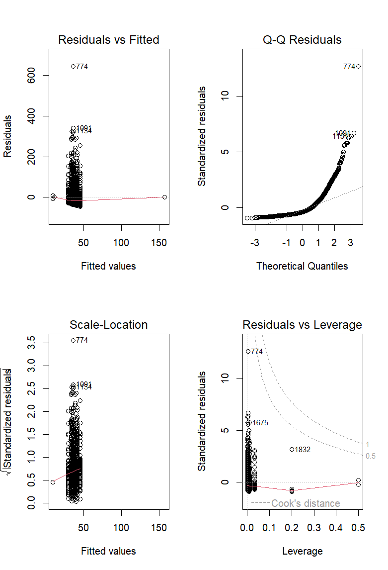
2.5.1 Interpretation and Conclusion
The linear regression model indicates that certain carriers significantly impact flight arrival delays. Specifically, carriers such as American Airlines, Delta Airlines, and United Airlines, among others, are associated with shorter arrival delays compared to the baseline carrier. However, the low R-squared value highlights that much of the variability in arrival delays remains unexplained by the carrier variable alone, suggesting the presence of other influential factors not included in this model. The diagnostic plots generally confirm the assumptions of the regression model but also point to the presence of potential outliers and influential points that may affect the model’s accuracy.