Chapter 5 Support Vector Machine
By Sheptim Veseli
5.1 Introduction
In our analysis, we apply the SVM algorithm to predict the log-transformed arrival delays of flights based on the carrier variable. The log transformation of arrival delays helps to stabilize variance and normalize the distribution, making it more suitable for regression modeling. The SVM model is trained on a subset of the flight data and evaluated on a separate test set to assess its predictive performance.
5.2 Data Preparation
The dataset was first prepared by removing any missing values to ensure the integrity of the analysis. The ‘carrier’ variable, representing different airlines, was converted into a factor to facilitate its use in the SVM model.
5.3 Training and Test Split
To evaluate the model’s performance, the dataset was split into training and test sets, with 80% of the data used for training the model and the remaining 20% reserved for testing.
# Set seed for reproducibility
set.seed(123)
# Split the data into training and test sets
train_index <- createDataPartition(flights_subset$log_arr_delay, p = 0.8, list = FALSE)
train_data <- flights_subset[train_index, ]
test_data <- flights_subset[-train_index, ]
5.3.1 SVM Model Training
The SVM model was trained using the svm function from the e1071 package, with the log-transformed arrival delay as the dependent variable and the carrier as the independent variable. The model employed the radial basis function (RBF) kernel, which is well-suited for capturing non-linear relationships.
# Train the SVM model
svm_model <- svm(log_arr_delay ~ carrier, data = train_data, type = "eps-regression")
Summary Preview
##
## Call:
## svm(formula = log_arr_delay ~ carrier, data = train_data, type = "eps-regression")
##
##
## Parameters:
##    SVM-Type:  eps-regression
##  SVM-Kernel:  radial
##        cost:  1
##       gamma:  0.06666667
##     epsilon:  0.1
##
##
## Number of Support Vectors:  1530
The SVM model parameters were as follows:
SVM-Type: epsilon-regression
SVM-Kernel: radial
Cost (C): 1
Gamma: 0.0667
Epsilon: 0.1
Number of Support Vectors: 1530
5.4 Model Evaluation
The model’s performance was evaluated on the test set. The Mean Squared Error (MSE) and Root Mean Squared Error (RMSE) were calculated to quantify the accuracy of the predictions.
## Mean Squared Error: 1.588177## Root Mean Squared Error: 1.260229The results were:
Mean Squared Error (MSE): 1.588
Root Mean Squared Error (RMSE): 1.260
These metrics indicate the average squared difference and the average error between the predicted and actual log-transformed arrival delays, respectively.
5.4.1 Result Interpretation
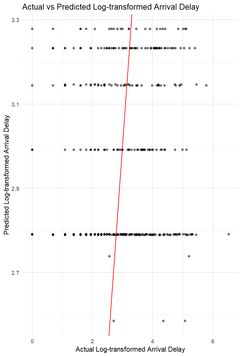
The scatter plot below illustrates the relationship between the actual and predicted log-transformed arrival delays. The red line represents the ideal scenario where the predicted values perfectly match the actual values. The proximity of the points to this line indicates the accuracy of the model’s predictions.
5.4.2 Discussion
The SVM model, with its radial basis function kernel, effectively captured the non-linear relationship between the carrier and the log-transformed arrival delay. The model’s performance, as indicated by the RMSE, suggests that while the SVM provides reasonably accurate predictions, there is still room for improvement. The scatter plot reveals that the predictions are closely aligned with the actual values, though some variability remains unaccounted for.
5.5 Conclusion
The application of Support Vector Machines to predict flight arrival delays demonstrates the utility of this machine learning technique in handling complex, non-linear relationships. The analysis shows that certain carriers have a measurable impact on arrival delays, though the low R-squared value in the initial linear regression suggests that other factors, such as weather conditions or airport congestion, likely play significant roles. Future work could involve incorporating additional predictors and exploring other machine learning algorithms to further enhance the model’s predictive power.